Last year I wrote a post about cubicaltt on this blog. Since then there have been a lot of exciting developments in the world of cubes. In particular there are now two cubical proof assistants that are currently being developed in Gothenburg and Pittsburgh. One of them is a cubical version of Agda developed by Andrea Vezzosi at Chalmers and the other is a system called redtt developed by my colleagues at CMU.
These systems differ from cubicaltt in that they are proper proof assistants for cubical type theory in the sense that they support unification, interactive proof development via holes, etc… Cubical Agda inherits Agda’s powerful dependent pattern matching functionality, and redtt has a succinct notation for defining functions by eliminators. Our goal with cubicaltt was never to develop yet another proof assistant, but rather to explore how it could be to program and work in a core system based on cubical type theory. This meant that many things were quite tedious to do in cubicaltt, so it is great that we now have these more advanced systems that are much more pleasant to work in.
This post is about Cubical Agda, but more or less everything in it can also be done (with slight modifications) in redtt. This extension of Agda has actually been around for a few years now, however it is just this year that the theory of HITs has been properly worked out for cubical type theory:
On Higher Inductive Types in Cubical Type Theory
Inspired by this paper (which I will refer as “CHM”) Andrea has extended Cubical Agda with user definable HITs with definitional computation rules for all constructors. Working with these is a lot of fun and I have been doing many of the proofs in synthetic homotopy theory from the HoTT book cubically. Having a system with native support for HITs makes many things a lot easier and most of the proofs I have done are significantly shorter. However, this post will not focus on HITs, but rather on a core library for Cubical Agda that we have been developing over the last few months:
https://github.com/agda/cubical
The core part of this library has been designed with the aim to:
1. Expose and document the cubical primitives of Agda.
2. Provide an interface to HoTT as presented in the book (i.e. “Book HoTT”), but where everything is implemented with the cubical primitives under the hood.
The idea behind the second of these was suggested to me by Martín Escardó who wanted a file which exposes an identity type with the standard introduction principle and eliminator (satisfying the computation rule definitionally), together with function extensionality, univalence and propositional truncation. All of these notions should be represented using cubical primitives under the hood which means that they all compute and that there are no axioms involved. In particular this means that one can import this file in an Agda developments relying on Book HoTT and no axioms should then be needed; more about this later.
Our cubical library compiles with the latest development version of Agda and it is currently divided into 3 main parts:
Cubical.Basics
Cubical.Core
Cubical.HITs
The first of these contain various basic results from HoTT/UF, like isomorphisms are equivalences (i.e. have contractible fibers), Hedberg’s theorem (types with decidable equality are sets), various proofs of different formulations of univalence, etc. This part of the library is currently in flux as I’m adding a lot of results to it all the time.
The second one is the one I will focus on in this post and it is supposed to be quite stable by now. The files in this folder expose the cubical primitives and the cubical interface to HoTT/UF. Ideally a regular user should not have to look too closely at these files and instead just import Cubical.Core.Everything or Cubical.Core.HoTT-UF.
The third folder contains various HITs (S¹, S², S³, torus, suspension, pushouts, interval, join, smash products…) with some basic theory about these. I plan to write another post about this soon, so stay tuned.
As I said above a regular user should only really need to know about the Cubical.Core.Everything and Cubical.Core.HoTT-UF files in the core library. The Cubical.Core.Everything file exports the following things:
-- Basic primitives (some are from Agda.Primitive)
open import Cubical.Core.Primitives public

-- Basic cubical prelude
open import Cubical.Core.Prelude public

-- Definition of equivalences, Glue types and
-- the univalence theorem
open import Cubical.Core.Glue public

-- Propositional truncation defined as a
-- higher inductive type
open import Cubical.Core.PropositionalTruncation public

-- Definition of Identity types and definitions of J,
-- funExt, univalence and propositional truncation
-- using Id instead of Path
open import Cubical.Core.Id public
I will explain the contents of the Cubical.Core.HoTT-UF file in detail later in this post, but I would first like to clarify that it is absolutely not necessary to use that file as a new user. The point of it is mainly to provide a way to make already existing HoTT/UF developments in Agda compute, but I personally only use the cubical primitives provided by the Cubical.Core.Everything file when developing something new in Cubical Agda as I find these much more natural to work with (especially when reasoning about HITs).
Cubical Primitives
It is not my intention to write another detailed explanation of cubical type theory in this post; for that see my previous post and the paper (which is commonly referred to as “CCHM”, after the authors of CCHM):
Cubical Type Theory: a constructive interpretation of the univalence axiom
The main things that the CCHM cubical type theory extends dependent type theory with are:
- An interval pretype
- Kan operations
- Glue types
- Cubical identity types
The first of these is what lets us work directly with higher dimensional cubes in type theory and incorporating this into the judgmental structure is really what makes the system tick. The Cubical.Core.Primitives and Cubical.Core.Prelude files provide 1 and 2, together with some extra stuff that are needed to get 3 and 4 up and running.
Let’s first look at the cubical interval I. It has endpoints i0 : I and i1 : I together with connections and reversals:
_∧_ : I → I → I
_∨_ : I → I → I
~_ : I → I
satisfying the structure of a De Morgan algebra (as in CCHM). As Agda doesn’t have a notion of non-fibrant types (yet?) the interval I lives in Setω.
There are also (dependent) cubical Path types:
PathP : ∀ {ℓ} (A : I → Set ℓ) → A i0 → A i1 → Set ℓ
from which we can define non-dependent Paths:
Path : ∀ {ℓ} (A : Set ℓ) → A → A → Set ℓ
Path A a b = PathP (λ _ → A) a b
A non-dependent path Path A a b gets printed as a ≡ b. I would like to generalize this at some point and have cubical extension types (inspired by A type theory for synthetic ∞-categories). These extension types are already in redtt and has proved to be very natural and useful, especially for working with HITs as shown by this snippet of redtt code coming from the proof that the loop space of the circle is the integers:
def decode-square
  : (n : int)
  → [i j] s1 [
    | i=0 → loopn (pred n) j
    | i=1 → loopn n j
    | j=0 → base
    | j=1 → loop i
    ]
  = ...
Just like in cubicaltt we get short proofs of the basic primitives from HoTT/UF:
refl : ∀ {ℓ} {A : Set ℓ} (x : A) → x ≡ x
refl x = λ _ → x

sym : ∀ {ℓ} {A : Set ℓ} {x y : A} → x ≡ y → y ≡ x
sym p = λ i → p (~ i)

cong : ∀ {ℓ ℓ'} {A : Set ℓ} {B : A → Set ℓ'} {x y : A}
         (f : (a : A) → B a)
         (p : x ≡ y) →
         PathP (λ i → B (p i)) (f x) (f y)
cong f p = λ i → f (p i)

funExt : ∀ {ℓ ℓ'} {A : Set ℓ} {B : A → Set ℓ'}
           {f g : (x : A) → B x}
           (p : (x : A) → f x ≡ g x) →
           f ≡ g
funExt p i x = p x i
Note that the proof of functional extensionality is just swapping the arguments to p!
Partial elements and cubical subtypes
[In order for me to be able to explain the other features of Cubical Agda in some detail I have to spend some time on partial elements and cubical subtypes, but as these notions are quite technical I would recommend readers who are not already familiar with them to just skim over this section and read it more carefully later.]
One of the key operations in the cubical set model is to map an element of the interval to an element of the face lattice (i.e. the type of cofibrant propositions F ⊂ Ω). This map is written (_ = 1) : I → F in CCHM and in Cubical Agda it is written IsOne r. The constant 1=1 is a proof that (i1 = 1), i.e. of IsOne i1.
This lets us then work with partial types and elements directly (which was not possible in cubicaltt). The type Partial φ A is a special version of the function space IsOne φ → A with a more extensional judgmental equality. There is also a dependent version PartialP φ A which allows A to be defined only on φ. As these types are not necessarily fibrant they also live in Setω. These types are easiest to understand by seeing how one can introduce them:
sys : ∀ i → Partial (i ∨ ~ i) Set₁
sys i (i = i1) = Set → Set
sys i (i = i0) = Set
This defines a partial type in Set₁ which is defined when (i = i1) ∨ (i = i0). We define it by pattern matching so that it is Set → Set when (i = i1) and Set when (i = i0). Note that we are writing (i ∨ ~ i) and that the IsOne map is implicit. If one instead puts a hole as right hand side:
sys : ∀ i → Partial (i ∨ ~ i) Set₁
sys i x = {! x !}
and ask Agda what the type of x is (by putting the cursor in the hole and typing C-c C-,) then Agda answers:
Goal: Set₁
—————————————————————————————————————————————
x : IsOne (i ∨ ~ i)
i : I
I usually introduce these using pattern matching lambdas so that I can write:
sys' : ∀ i → Partial (i ∨ ~ i) Set₁
sys' i = \ { (i = i0) → Set
           ; (i = i1) → Set → Set }
This is very convenient when using the Kan operations. Furthermore, when the cases overlap they must of course agree:
sys2 : ∀ i j → Partial (i ∨ (i ∧ j)) Set₁
sys2 i j = \ { (i = i1) → Set
             ; (i = i1) (j = i1) → Set }
In order to get this to work Andrea had to adapt the pattern-matching of Agda to allow us to pattern-match on the faces like this. It is however not yet possible to use C-c C-c to automatically generate the cases for a partial element, but hopefully this will be added at some point.
Using the partial elements there are also cubical subtypes as in CCHM:
_[_↦_] : ∀ {ℓ} (A : Set ℓ) (φ : I) (u : Partial φ A) →
         Agda.Primitive.Setω
A [ φ ↦ u ] = Sub A φ u
So that a : A [ φ ↦ u ] is a partial element a : A that agrees with u on φ. We have maps in and out of the subtypes:
inc : ∀ {ℓ} {A : Set ℓ} {φ} (u : A) →
        A [ φ ↦ (λ _ → u) ]

ouc : ∀ {ℓ} {A : Set ℓ} {φ : I} {u : Partial φ A} →
        A [ φ ↦ u ] → A
It would be very nice to have subtyping for these, but at the moment the user has to write inc/ouc explicitly. With this infrastructure we can now consider the Kan operations of cubical type theory.
Kan operations
In order to support HITs we use the Kan operations from CHM. The first of these is a generalized transport operation:
transp : ∀ {ℓ} (A : I → Set ℓ) (φ : I) (a : A i0) → A i1
When calling transp A φ a Agda makes sure that A is constant on φ and when calling this with i0 for φ we recover the regular transport function, furthermore when φ is i1 this is the identity function. Being able to control when transport is the identity function is really what makes this operation so useful (see the definition of comp below) and why we got HITs to work so nicely in CHM compared to CCHM.
We also have homogeneous composition operations:
hcomp : ∀ {ℓ} {A : Set ℓ} {φ : I}
          (u : I → Partial A φ) (a : A) → A
When calling hcomp A φ u a Agda makes sure that a agrees with u i0 on φ. This is like the composition operations in CCHM, but the type A is constant. Note that this operation is actually different from the one in CHM as φ is in the interval and not the face lattice. By the way the partial elements are set up the faces will then be compared under the image of IsOne. This subtle detail is actually very useful and gives a very neat trick for eliminating empty systems from Cubical Agda (this has not yet been implemented, but it is discussed here).
Using these two operations we can derive the heterogeneous composition
operation:
comp : ∀ {ℓ : I → Level} (A : ∀ i → Set (ℓ i)) {φ : I}
         (u : ∀ i → Partial φ (A i))
         (u0 : A i0 [ φ ↦ u i0 ]) → A i1
comp A {φ = φ} u u0 =
  hcomp
    (λ i → λ { (φ = i1) →
                 transp (λ j → A (i ∨ j)) i (u _ 1=1) })
    (transp A i0 (ouc u0))
This decomposition of the Kan operations into transport and homogeneous composition seems crucial to get HITs to work properly in cubical type theory and in fact redtt is also using a similar decomposition of their Kan operations.
We can also derive both homogeneous and heterogeneous Kan filling using hcomp and comp with connections:
hfill : ∀ {ℓ} {A : Set ℓ} {φ : I}
         (u : ∀ i → Partial φ A)
         (u0 : A [ φ ↦ u i0 ])
         (i : I) → A
hfill {φ = φ} u u0 i =
  hcomp (λ j → λ { (φ = i1) → u (i ∧ j) 1=1
                 ; (i = i0) → ouc u0 })
        (ouc u0)

fill : ∀ {ℓ : I → Level} (A : ∀ i → Set (ℓ i)) {φ : I}
        (u : ∀ i → Partial φ (A i))
        (u0 : A i0 [ φ ↦ u i0 ])
        (i : I) → A i
fill A {φ = φ} u u0 i =
  comp (λ j → A (i ∧ j))
       (λ j → λ { (φ = i1) → u (i ∧ j) 1=1
                ; (i = i0) → ouc u0 })
       (inc {φ = φ ∨ (~ i)} (ouc {φ = φ} u0))
Using these operations we can do all of the standard cubical stuff, like composing paths and defining J with its computation rule (up to a Path):
compPath : ∀ {ℓ} {A : Set ℓ} {x y z : A} →
             x ≡ y → y ≡ z → x ≡ z
compPath {x = x} p q i =
  hcomp (λ j → \ { (i = i0) → x
                 ; (i = i1) → q j })
        (p i)

module _ {ℓ ℓ'} {A : Set ℓ} {x : A}
         (P : ∀ y → x ≡ y → Set ℓ') (d : P x refl) where
  J : {y : A} → (p : x ≡ y) → P y p
  J p = transp (λ i → P (p i) (λ j → p (i ∧ j))) i0 d

  JRefl : J refl ≡ d
  JRefl i = transp (λ _ → P x refl) i d
The use of a module here is not crucial in any way, it’s just an Agda trick to make J and JRefl share some arguments.
Glue types and univalence
The file Cubical.Core.Glue defines fibers and equivalences (as they were originally defined by Voevodsky in his Foundations library, i.e. as maps with contractible fibers). Using this we export the Glue types of Cubical Agda which lets us extend a total type by a partial family of equivalent types:
Glue : ∀ {ℓ ℓ'} (A : Set ℓ) {φ : I} →
         (Te : Partial φ (Σ[ T ∈ Set ℓ' ] T ≃ A)) →
         Set ℓ'
This comes with introduction and elimination forms (glue and unglue). With this we formalize the proof of a variation of univalence following the proof in Section 7.2 of CCHM. The key observation is that unglue is an equivalence:
unglueIsEquiv : ∀ {ℓ} (A : Set ℓ) (φ : I)
                  (f : PartialP φ (λ o → Σ[ T ∈ Set ℓ ] T ≃ A)) →
                  isEquiv {A = Glue A f} (unglue {φ = φ})
equiv-proof (unglueIsEquiv A φ f) = λ (b : A) →
  let u : I → Partial φ A
      u i = λ{ (φ = i1) → equivCtr (f 1=1 .snd) b .snd (~ i) }
      ctr : fiber (unglue {φ = φ}) b
      ctr = ( glue (λ { (φ = i1) → equivCtr (f 1=1 .snd) b .fst }) (hcomp u b)
            , λ j → hfill u (inc b) (~ j))
  in ( ctr
     , λ (v : fiber (unglue {φ = φ}) b) i →
         let u' : I → Partial (φ ∨ ~ i ∨ i) A
             u' j = λ { (φ = i1) → equivCtrPath (f 1=1 .snd) b v i .snd (~ j)
                      ; (i = i0) → hfill u (inc b) j
                      ; (i = i1) → v .snd (~ j) }
         in ( glue (λ { (φ = i1) → equivCtrPath (f 1=1 .snd) b v i .fst }) (hcomp u' b)
            , λ j → hfill u' (inc b) (~ j)))
The details of this proof is best studied interactively in Agda and by first understanding the proof in CCHM. The reason this is a crucial observation is that it says that any partial family of equivalences can be extended to a total one from Glue [ φ ↦ (T,f) ] A to A:
unglueEquiv : ∀ {ℓ} (A : Set ℓ) (φ : I)
              (f : PartialP φ (λ o → Σ[ T ∈ Set ℓ ] T ≃ A)) →
              (Glue A f) ≃ A
unglueEquiv A φ f = ( unglue {φ = φ} , unglueIsEquiv A φ f )
and this is exactly what we need to prove the following formulation of the univalence theorem:
EquivContr : ∀ {ℓ} (A : Set ℓ) → isContr (Σ[ T ∈ Set ℓ ] T ≃ A)
EquivContr {ℓ} A =
  ( ( A , idEquiv A)
  , λ w i →
      let f : PartialP (~ i ∨ i) (λ x → Σ[ T ∈ Set ℓ ] T ≃ A)
          f = λ { (i = i0) → ( A , idEquiv A ) ; (i = i1) → w }
      in ( Glue A f , unglueEquiv A (~ i ∨ i) f) )
This formulation of univalence was proposed by Martín Escardó in (see also Theorem 5.8.4 of the HoTT Book):
https://groups.google.com/forum/#!msg/homotopytypetheory/HfCB_b-PNEU/Ibb48LvUMeUJ
We have also formalized a quite slick proof of the standard formulation of univalence from EquivContr (see Cubical.Basics.Univalence). This proof uses that EquivContr is contractibility of singletons for equivalences, which combined with subst can be used to prove equivalence induction:
contrSinglEquiv : ∀ {ℓ} {A B : Set ℓ} (e : A ≃ B) →
                    (B , idEquiv B) ≡ (A , e)
contrSinglEquiv {A = A} {B = B} e =
  isContr→isProp (EquivContr B) (B , idEquiv B) (A , e)

EquivJ : ∀ {ℓ ℓ′} (P : (A B : Set ℓ) → (e : B ≃ A) → Set ℓ′)
           (r : (A : Set ℓ) → P A A (idEquiv A))
           (A B : Set ℓ) (e : B ≃ A) →
           P A B e
EquivJ P r A B e =
  subst (λ x → P A (x .fst) (x .snd))
        (contrSinglEquiv e) (r A)
We then use that the Glue types also gives a map ua which maps the identity equivalence to refl:
ua : ∀ {ℓ} {A B : Set ℓ} → A ≃ B → A ≡ B
ua {A = A} {B = B} e i =
  Glue B (λ { (i = i0) → (A , e)
            ; (i = i1) → (B , idEquiv B) })

uaIdEquiv : ∀ {ℓ} {A : Set ℓ} → ua (idEquiv A) ≡ refl
uaIdEquiv {A = A} i j =
  Glue A {φ = i ∨ ~ j ∨ j} (λ _ → A , idEquiv A)
Now, given any function au : ∀ {ℓ} {A B : Set ℓ} → A ≡ B → A ≃ B satisfying auid : ∀ {ℓ} {A B : Set ℓ} → au refl ≡ idEquiv A we directly get that this is an equivalence using the fact that any isomorphism is an equivalence:
module Univalence
         (au : ∀ {ℓ} {A B : Set ℓ} → A ≡ B → A ≃ B)
         (auid : ∀ {ℓ} {A B : Set ℓ} → au refl ≡ idEquiv A) where
  thm : ∀ {ℓ} {A B : Set ℓ} → isEquiv au
  thm {A = A} {B = B} =
    isoToIsEquiv {B = A ≃ B} au ua
      (EquivJ (λ _ _ e → au (ua e) ≡ e)
              (λ X → compPath (cong au uaIdEquiv)
                              (auid {B = B})) _ _)
      (J (λ X p → ua (au p) ≡ p)
         (compPath (cong ua (auid {B = B})) uaIdEquiv))
We can then instantiate this with for example the au map defined using J (which is how Vladimir originally stated the univalence axiom):
eqweqmap : ∀ {ℓ} {A B : Set ℓ} → A ≡ B → A ≃ B
eqweqmap {A = A} e = J (λ X _ → A ≃ X) (idEquiv A) e

eqweqmapid : ∀ {ℓ} {A : Set ℓ} → eqweqmap refl ≡ idEquiv A
eqweqmapid {A = A} = JRefl (λ X _ → A ≃ X) (idEquiv A)

univalenceStatement : ∀ {ℓ} {A B : Set ℓ} →
                      isEquiv (eqweqmap {ℓ} {A} {B})
univalenceStatement = Univalence.thm eqweqmap eqweqmapid
Note that eqweqmapid is not proved by refl, instead we need to use the fact that the computation rule for J holds up to a Path. Furthermore, I would like to emphasize that there is no problem with using J for Path’s and that the fact that the computation rule doesn’t hold definitionally is almost never a problem for practical formalization as one rarely use it as it is often more natural to just use the cubical primitives. However, in Section 9.1 of CCHM we solve this by defining cubical identity types satisfying the computation rule definitionally (following a trick of Andrew Swan).
Cubical identity types
The idea behind the cubical identity types is that an element of an identity type is a pair of a path and a formula which tells us where this path is constant, so for example reflexivity is just the constant path together with the fact that it is constant everywhere (note that the interval variable comes before the path as the path depends on it):
refl : ∀ {ℓ} {A : Set ℓ} {x : A} → Id x x
refl {x = x} = ⟨ i1 , (λ _ → x) ⟩
These types also come with an eliminator from which we can prove J such that it is the identity function on refl, i.e. where the computation rule holds definitionally (for details see the Agda code in Cubical.Core.Id). We then prove that Path and Id are equivalent types and develop the theory that we have for Path for Id as well, in particular we prove the univalence theorem expressed with Id everywhere (the usual formulation can be found in Cubical.Basics.UnivalenceId).
Note that the cubical identity types are not an inductive family like in HoTT which means that we cannot use Agda’s pattern-matching to match on them. Furthermore Cubical Agda doesn’t support inductive families yet, but it should be possible to adapt the techniques of Cavallo/Harper presented in
Higher Inductive Types in Cubical Computational Type Theory
in order to extend it with inductive families. The traditional identity types could then be defined as in HoTT and pattern-matching should work as expected.
Propositional truncation
The core library only contains one HIT: propositional truncation (Cubical.Core.PropositionalTruncation). As Cubical Agda has native support for user defined HITs this is very convenient to define:
data ∥_∥ {ℓ} (A : Set ℓ) : Set ℓ where
  ∣_∣ : A → ∥ A ∥
  squash : ∀ (x y : ∥ A ∥) → x ≡ y
We can then prove the recursor (and eliminator) using pattern-matching:
recPropTrunc : ∀ {ℓ} {A : Set ℓ} {P : Set ℓ} →
                 isProp P → (A → P) → ∥ A ∥ → P
recPropTrunc Pprop f ∣ x ∣          = f x
recPropTrunc Pprop f (squash x y i) =
  Pprop (recPropTrunc Pprop f x) (recPropTrunc Pprop f y) i
However I would not only use recPropTrunc explicitly as we can just use pattern-matching to define functions out of HITs. Note that the cubical machinery makes it possible for us to define these pattern-matching equations in a very nice way without any ap‘s. This is one of the main reasons why I find it a lot more natural to work with HITs in cubical type theory than in Book HoTT: the higher constructors of HITs construct actual elements of the HIT, not of its identity type!
This is just a short example of what can be done with HITs in Cubical Agda, I plan to write more about this in a future post, but for now one can look at the folder Cubical/HITs for many more examples (S¹, S², S³, torus, suspension, pushouts, interval, join, smash products…).
Constructive HoTT/UF
By combining everything I have said so far we have written the file Cubical.Core.HoTT-UF which exports the primitives of HoTT/UF defined using cubical machinery under the hood:
open import Cubical.Core.Id public
     using ( _≡_            -- The identity type.
           ; refl           -- Unfortunately, pattern matching on refl is not available.
           ; J              -- Until it is, you have to use the induction principle J.
           ; transport      -- As in the HoTT Book.
           ; ap
           ; _∙_
           ; _⁻¹
           ; _≡⟨_⟩_         -- Standard equational reasoning.
           ; _∎
           ; funExt         -- Function extensionality
                            -- (can also be derived from univalence).
           ; Σ              -- Sum type. Needed to define contractible types, equivalences
           ; _,_            -- and univalence.
           ; pr₁            -- The eta rule is available.
           ; pr₂
           ; isProp         -- The usual notions of proposition, contractible type, set.
           ; isContr
           ; isSet
           ; isEquiv        -- A map with contractible fibers
                            -- (Voevodsky's version of the notion).
           ; _≃_            -- The type of equivalences between two given types.
           ; EquivContr     -- A formulation of univalence.
           ; ∥_∥             -- Propositional truncation.
           ; ∣_∣             -- Map into the propositional truncation.
           ; ∥∥-isProp       -- A truncated type is a proposition.
           ; ∥∥-recursion    -- Non-dependent elimination.
           ; ∥∥-induction    -- Dependent elimination.
           )
The idea is that if someone has some code written using HoTT/UF axioms in Agda they can just import this file and everything should compute properly. The only downside is that one has to rewrite all pattern-matches on Id to explicit uses of J, but if someone is willing to do this and have some cool examples that now compute please let me know!
That’s all I had to say about the library for now. Pull-requests and feedback on how to improve it are very welcome! Please use the Github page for the library for comments and issues:
https://github.com/agda/cubical/issues
If you find some bugs in Cubical Agda you can use the Github page of Agda to report them (just check that no-one has already reported the bug):
https://github.com/agda/agda/issues
 such that
  , as defined in
  such that the image
  of
of  under the equivalence
  satisfies
  . This is all incredibly impressive, and, naturally, it’s great to see that we can actually rephrase so many classical results in HoTT. Undoubtedly, the argument shows why the equivalence
  , but it doesn’t really tell us (explicitly) how this happens.
 .
.  — elements of other homotopy groups which the equivalence
  under the equivalence in question. The neat thing here is that the sequence gives rise to a sequence of new definitions of the Brunerie number, in decreasing level of ‘complexity’. The numbers corresponding to
  and
and  are still too heavy for Cubical Agda to handle, but (an optimised version of)
  normalises to
  . We define it using the standard
  construction:

 using the following constructors:


 using the following constructors:

 -fold suspension of
  . We take
  and higher spheres to be pointed by
  . Another type of interest,
  , will be taken to be pointed by
  . Given a pointed type
  , we define its
  , i.e. the set truncated type of pointed functions from
  to
to  to denote addition on
  to denote inversion on arbitrary
  for the canonical function
  (where

 . In HoTT, we can define it by
  and
and 
 is suggestive – it satisfies most properties that you’d expect from a ‘cup product’ (in fact it induces a ‘true’ cup product via the map
  ). It satisfies the following properties, all provable by circle induction:
 by
by


 via joins
 with a not so nice map, namely
  . However, what if we defined
  instead? Clearly, this definition is equivalent to the usual one by precomposition with
  . This would allow us redefine the Brunerie map to be simply
  . Let’s make this happen.
 , we get an induced map
  defined by
 when
when  in
in  is induced by the composition
  .
. -connected) to show that
  . This is the key to understanding
  . In the first 3 chapters of Brunerie’s thesis, he shows that
  where
where  and where
  . It’s probably time to define


 .
. ,
,  as a composition of 4 group isomorphisms
  and simultaneously tracing
 — it comes from the long exact sequence of homotopy groups induced from the Hopf fibration. Fortunately, however, its inverse is easy to describe: it is simply postcomposition with the Hopf map
  . The Hopf map is defined as follows:

 such that
  . It is defined as follows:


 . For this, we need to show that
  . I won’t do this here, but the proof is very direct. The idea is that the terms in the
  -case are chosen precisely to take care of the
  appearing in the definition of the Hopf map.
 is defined by postcomposition with
  . It is defined by


 . To prove this, we need to show that
  . Let’s consider the definition of
  (modulo some light rewriting):


 .
.
 is straightforward. I won’t do this here, but the idea is that by following
  under
under  , we see that
  . In fact, we can also show that (a slight rephrasing of)
  is
is  .
. . However, it is enough to show that
 , then
  -torsion in
  . It is defined by

 . In other words, if we could flip the two path components in the definition of
  . Naturally, this is not possible. But what happens if we suspend the situation?
 induces a surjection
  . We can easily show that
  : for point constructors it holds definitionally and for the
 , and thus the Eckmann-Hilton argument applies, making the above equation hold. So the surjection
  takes
takes  in the formalisation — sorry!). I suspect that the argument shouldn’t be much harder to formalise in standard Agda or Coq.
 , the
, the  -topos theory and in HoTT/UF, where in the latter a truth value is a type with at most one element, also known as a proposition (and sometimes as an h-proposition or as a mere proposition).
 is an involution, that is,
  .
. on
on  for every
 ,
,  , or any element of
  .
.


 .
. by propositional extensionality (or univalence for propositions, in the case of HoTT/UF).
 , and
, and
 and
and ![[0,1]](https://s0.wp.com/latex.php?latex=%5B0%2C1%5D&bg=ffffff&fg=333333&s=0&c=20201002) are order-embedded into each other, but they are not order isomorphic.
are order-embedded into each other, but they are not order isomorphic. is an injection if and only if it is left-cancellable, in the sense that
  implies
  . But, for types
  and
and  that are not sets, this notion is too weak, and, moreover, is not a proposition as the identity type
  has multiple elements in general. The appropriate notion of embedding for a function
  is an equivalence for any
  .
. that picks a point
  is left-cancellable, but it is an embedding if and only if the point
  is homotopy isolated, which amounts to saying that the identity type
  is contractible. This fails, for instance, when the type
  be embeddings of arbitrary types
  is a
is a  and
and  with
with  , the
, the  is inhabited. Using function extensionality and the assumption that
  and
and  , we see that if
  is a
is a  of
of  . In particular if
  is a
is a  , and because
  .
. by
by  if
if  , otherwise.
  is left-cancellable and split-surjective, as any such map is an equivalence.
 be a
be a  . Then
  . Now, because if
  were a
  is an
is an  of the
  in the
  . By the axioms of differential cohesion, it has a left and a right adjoint and is idempotent. These properties are more than enough to model a monadic modality in homotopy type theory. Monadic modalities were already defined at the end of section 7 in the HoTT-Book and named just “modalities” and it is possible to have a homotopy type theory with a monadic modality just by adding some axioms — which is known not to work for non-trivial comonadic modalities.
 and a unit
 on some type
  are equivalences for all
 . This makes sense if we think of some very special interpretations of
  is given as the quotient map from a space
  by a relation that identifies infinitesimally close points in
  being infinitesimally close, denoted “
 ” in terms of the units:
 ” denotes the identity type (of
  :
:
 preserves inifinitesimal closeness, i.e.

 are also equivalences. The latter corresponds to the fact that the differential of a diffeomorphism is invertible.
 are a family of equivalences that consistently identify
  with all other formal disks
  .
.
 .
. -types, identity types, “large”
  -types over an impredicative universe
  and function extensionality. Having large
  and a type family
  , we may form the dependent function type
 (or alternatively over the subtype of
 is given by
 -algebras:
 and
and  :
:
 .
. and moreover let
  be the forgetful functor to
  be the covariant Yoneda embedding. We reason as follows:
 is defined as a limit, we obtain an algebra structure
  . As
. As  is guaranteed to be initial in
 . Impredicativity is crucial for this: it guarantees that the product over
  ! We won’t pursue this remarkable fact here, but only consider the case at hand, where the functor
  becomes our definition of the type of natural numbers (so let us rename
  for the remainder). Observe that this encoding can be seen as a subtype of (a translation of) the System F encoding given at the start. Indeed, the indexing object
  of
of  , by
, by

 , given any
  and
and  . In other words, the introduction rules hold, and we can eliminate into other sets. Further, the
  such that:
 . Then

 with fixed endpoints.
 is a class function, assigning to any set
  , then the image of any set
  is again a set. In homotopy type theory we consider instead a map
  from a small type
  into a locally small type
  with the universal property of the image of
  , and let
  be a type with
  . Then the following are equivalent.
 is contractible.
 defined by path induction, mapping
  to
to  , is a fiberwise equivalence.
 . In other words,
  is in the connected component of the type family
  .
. and an equivalence
  .
. , and the canonical dependent function
  defined by path induction by sending
  to
to  is an equivalence.
 , while the equivalences in the second structure are canonical with respect to the choice of reflexivity
  is contractible. Thus we see by Licata’s theorem that the canoncial fiberwise map is a fiberwise equivalence. Furthermore, it is not hard to see that the family of equivalences
  is equal to the canonical family of equivalences. There is slightly more to show, but let us keep up the pace and go on.
 is locally small. Observe also that the univalence axiom follows if we assume the `uncanonical univalence axiom’, namely that there merely exists a family of equivalences
  . Thus we see that the slogan ‘identity of the universe is equivalent to equivalence’ actually implies univalence.
 . Then we can construct
 ,
,
 is an embedding that satisfies the universal property of the image inclusion, namely that for any embedding
  for the mere proposition that
 is defined by first pulling back, and then taking the pushout, as indicated in the following diagram
 , the type
  is equivalent to the usual join of types
  . Just like the join of types, the join of maps with a common codomain is associative, commutative, and it has a unit: the unique map from the empty type into
  in the slice category over
  on any univalent universe that is closed under pushouts. Other applications include the construction of set-quotients and of Rezk-completion, since these are both constructed as the image of the Yoneda-embedding, and it also follows that the univalent completion of any dependent type
  can be constructed as a type in
  , without needing to resort to more exotic higher inductive types. In particular, any connected component of the universe is equivalent to a small type.
 ,
, 
 is n-truncated and satisfies the (dependent) universal property of n-truncation, namely that for every type family
  of possibly large types such that each
  is n-truncated, the canonical map
 is an equivalence.
 is trivial (take
  ). For the induction hypothesis we assume an n-truncation operation with structure described in the statement of the theorem.
 by
by  . As we have seen, the universe is locally small, and therefore the type
  is locally small. Therefore we can define
 .
. is indeed
  -truncated, and satisfies the universal property of the n-truncation we refer to the article.
 of polymorphic endomaps is the polymorphic identity
  .
. is the flip map on the type of booleans, then excluded middle holds. In the paper on arXiv, we have a stronger result:
 if and only if excluded middle holds.
 and types
  and points
  with
with  if and only if weak excluded middle holds.
 , and otherwise we map
  for any proposition, so this is an automorphism.
 with the unit type
  and leaves all other types unchanged. More generally, assuming excluded middle we can swap any two types with equivalent automorphism ∞-groups, since in that case the corresponding connected components of the universe are equivalent. Still more generally, we can permute arbitrarily any family of types all having the same automorphism ∞-group.
 is a group that is a set (i.e. a 1-group), then its Eilenberg-Mac Lane space
  is a 1-type, and its automorphism ∞-group is a 1-type whose
  is the outer automorphisms of
  is the center of
  is rigid. Such groups are not uncommon, including for instance the symmetric group
  for any
  . Thus, assuming excluded middle we can permute these
  arbitrarily, producing uncountably many automorphisms of the universe.
 of the universe with
  , then the double negation
 such that
  for a particular
  you get a non-provable consequence of excluded middle, then you get
  -many beers, where
  we have
  . Suppose
  with
with  , then
  . For suppose that
  , and hence
  . So by the corollary, we obtain
  . But
. But  implies
  , where
  is the groupoid of finite sets and bijections, and
  is the category of finite sets and (total) functions. Intuitively, we can think of a species as mapping finite sets of “labels” to finite sets of “structures” built from those labels. For example, the species of linear orderings (i.e. lists) maps the finite set of labels
  to the size-
 set of all possible linear orderings of those labels. Functoriality ensures that the specific identity of the labels does not matter—we can always coherently relabel things.
 can be represented by functions
  , that is, each natural number maps to some coefficient in
  ,
,
 . The only bijection which is allowed is the one which sends each element related to
  to the other element related to
  .
.
 instead of
  .) A few observations:
 . Intuitively, this is because if a set is finite, there is only one possible size it can have, so the evidence that it has that size is actually a mere proposition.
 , since this reveals something about the underlying bijection; but we can write a function which finds the smallest value of
  itself is a 1-type.
 is really just a path
  between 0-types, that is, a bijection, since
  trivially.
 . The main reason I think this is the Right Definition ™ of species in HoTT is that functoriality comes for free! When defining species in set theory, one must say “a species is a functor, i.e. a pair of mappings satisfying such-and-such properties”. When constructing a particular species one must explicitly demonstrate the functoriality properties; since the mappings are just functions on sets, it is quite possible to write down mappings which are not functorial. But in HoTT, all functions are functorial with respect to paths, and we are using paths to represent the morphisms in
  is a groupoid,
  a category, and
  , then
  . In set theory, this coend would be a quotient of the corresponding
  such that
  is a non-identity function
  I have proved the converse of this. Like in exercise 6.9, we assume univalence.
 ?
? (Notice that the proof of this is not quite as trivial as it may seem: LEM only gives us
  if
if  does not work, because this is not necessarily a proposition.)
 with
with  then LEM holds.
 we can find an explicit boolean
  such that
  Without loss of generality, we can assume
 to prove LEM.
 and it can be defined as
  where
where  is the suspension of
  and also
 (not
(not  itself!). Now the proof continues by defining
 is the equivalence given by the identity function on
  ) and doing case analysis on
  and if necessary also on
  for some elements
  I do not believe it is very instructive to spell out all cases explicitly here. I wrote a more
  In particular, we do not require decidable equality of
  Assume
  then by transporting along an appropriate equivalence (namely the one that identifies
  with
with  we get
  But since
  is a fixed point,
  which is a contradiction.
 we can construct a diagram
 is defined by:
 is defined recursively from
  . We call this diagram the iterated kernel pair of
  . The result is that the colimit of this diagram is
  , the image of
  is
is  the homotopy fiber of
  (where
  is
is  the one-step truncation of
  the truncation of
  is the circle. We try to address this issue considering an HIT that take care of already existing paths:
 and the Čech nerve of a function. We outline this in the
  .
. :
: be a cocone into
  . Then we can extend
  to a cocone into
  by postcomposition with
 over the same diagram,
  if there exists a universal cocone over
  is a colimit of
  be two diagrams over the same graph
  is an equivalence of diagrams if all functions
  are equivalences. In that case, we can define the inverse of
  , we can make every cocone over


 given by
  is well an inverse of
  .
. we get:
 and
and  be two colimits of the same diagram, then:
  .
. be a type and, for all
  ,
,  a diagram over a graph
  and functions
  are induced by the identity on the first component and by
  on the second one. Let’s note
  this diagram.
 , we can make a cocone over
  .
.
 ,
,  is a colimit of
  , then
  is not strong enough. But we have the following result:
 (we will recover the theorem considering the unique function
  ).
). the colimit of the kernel pair of
 is given by
  .
.
 by universality (another point of view is to say that
  is defined by
 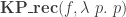 ).
).
 and
and  .
. , the image of
 (for
(for  ) at each type. Going from the second to the third is more involved, we don’t detail it here. And
  is the colimit of the diagram
 (which is
  (♣)
(♣) .
. then
then  and
and  are not equal. But now they become equal: by path induction we bring back to
  . That is, if two elements are already equal, we don’t add any path between them.
 is
is  is an equivalence for all
  ) then so is
  . In particular, if
  (meaning that the one-step truncation of an hProp is now itself).
 could be the colimit of the (n+1)-truncated Čech nerve. We are far from having such a proof but we succeeded in proving :
 is the colimit of the kernel pair (♣),
 doesn’t have such a compatibility: if
  and
and  , in general we do not have
 in
in  .
. in
in  .
. because
  is
is  .)
.) , and I want to write this blog post in case someone could not attend the talk but is interested nevertheless. There are also
  ?
?
 -limits (“infinite
  as the type of natural transformations between type-valued presheaves. If the type theory has propositional truncations, we can construct a canonical map from
  and
and  .
. ? If we think of elements of
  as anonymous inhabitants of
  which “cannot look at its input”. But then, how can we specify what it means to “not look at its input” internally? A first attempt could be requesting that
  . Indeed, it has been shown:
 , where the function from left to right is the canonical one.
  , we can try to fix the problem that the paths given by
  “do not fit together” by throwing in a coherence proof, i.e. an element of
  . We should already know that this will introduce its own problems and thus not fix everything, but at least, we get:
 , again given by a canonical map from left to right.
  . The type


 .
. . By going through the construction step-by-step, we see that the function part of the equivalence (map from left to right) is the canonical one (let’s write
  ), mapping
  to the triple
  . Before we have started the construction, we have assumed a point
  ! So, if the assumption
  . We can move the
  -part to both sides of the equivalence, and on the right-hand side, we can apply the usual “distributivity of
  )”, to move the
  and
and  are equivalent), which gives us the claimed result.
 -component is well-behaved). The core idea is that this expanding and contracting strategy can be done for any truncation level of
  and
and  and
and  we used in the special case can be seen as components of a natural transformation between
 ![[2]](https://s0.wp.com/latex.php?latex=%5B2%5D&bg=ffffff&fg=333333&s=0&c=20201002) -truncated semi-simplicial types. By semi-simplicial type, I mean a Reedy fibrant diagram
-truncated semi-simplicial types. By semi-simplicial type, I mean a Reedy fibrant diagram  . By
. By 
 , and its initial part is given by
 ![T \! A_{[0]} :\equiv A](https://s0.wp.com/latex.php?latex=T+%5C%21+A_%7B%5B0%5D%7D+%3A%5Cequiv+A&bg=ffffff&fg=333333&s=0&c=20201002) ,
, ![T \! A_{[1]} :\equiv A \times A](https://s0.wp.com/latex.php?latex=T+%5C%21+A_%7B%5B1%5D%7D+%3A%5Cequiv+A+%5Ctimes+A&bg=ffffff&fg=333333&s=0&c=20201002) , and
, and ![T \! A_{[2]} :\equiv A \times A \times A](https://s0.wp.com/latex.php?latex=T+%5C%21+A_%7B%5B2%5D%7D+%3A%5Cequiv+A+%5Ctimes+A+%5Ctimes+A&bg=ffffff&fg=333333&s=0&c=20201002) . If we use the “fibred” notation (i.e. give the fibres over the matching objects), this would be
. If we use the “fibred” notation (i.e. give the fibres over the matching objects), this would be ![T \! A_{[1]}(a_1,a_2) :\equiv \mathbf{1}](https://s0.wp.com/latex.php?latex=T+%5C%21+A_%7B%5B1%5D%7D%28a_1%2Ca_2%29+%3A%5Cequiv+%5Cmathbf%7B1%7D&bg=ffffff&fg=333333&s=0&c=20201002) ,
, ![T \! A_{[2]}(a_1,a_2,a_3,\_,\_,\_) :\equiv \mathbf{1}](https://s0.wp.com/latex.php?latex=T+%5C%21+A_%7B%5B2%5D%7D%28a_1%2Ca_2%2Ca_3%2C%5C_%2C%5C_%2C%5C_%29+%3A%5Cequiv+%5Cmathbf%7B1%7D&bg=ffffff&fg=333333&s=0&c=20201002) . In the terminology of simplicial sets, this is the
. In the terminology of simplicial sets, this is the ![[0]](https://s0.wp.com/latex.php?latex=%5B0%5D&bg=ffffff&fg=333333&s=0&c=20201002) -coskeleton of [the diagram that is constantly]
-coskeleton of [the diagram that is constantly]  . One potential definition for the lowest levels would be given by (I only give the fibres this time):
 ![E \! B_{[0]} :\equiv B](https://s0.wp.com/latex.php?latex=E+%5C%21+B_%7B%5B0%5D%7D+%3A%5Cequiv+B&bg=ffffff&fg=333333&s=0&c=20201002) ,
, ![E \! B_{[1]}(b_1,b_2) :\equiv b_1 = b_2](https://s0.wp.com/latex.php?latex=E+%5C%21+B_%7B%5B1%5D%7D%28b_1%2Cb_2%29+%3A%5Cequiv+b_1+%3D+b_2&bg=ffffff&fg=333333&s=0&c=20201002) ,
, ![E \! B_{[2]}(b_1,b_2,b_3,p_{12},p_{23},p_{13}) :\equiv p_{12} \cdot p_{23} = p_{13}](https://s0.wp.com/latex.php?latex=E+%5C%21+B_%7B%5B2%5D%7D%28b_1%2Cb_2%2Cb_3%2Cp_%7B12%7D%2Cp_%7B23%7D%2Cp_%7B13%7D%29+%3A%5Cequiv+p_%7B12%7D+%5Ccdot+p_%7B23%7D+%3D+p_%7B13%7D&bg=ffffff&fg=333333&s=0&c=20201002) . This is a fibrant replacement of
. This is a fibrant replacement of  with objects
 ![[0],[1],[2]](https://s0.wp.com/latex.php?latex=%5B0%5D%2C%5B1%5D%2C%5B2%5D&bg=ffffff&fg=333333&s=0&c=20201002) ) is, it is easy to see that the
) is, it is easy to see that the ![[1]](https://s0.wp.com/latex.php?latex=%5B1%5D&bg=ffffff&fg=333333&s=0&c=20201002) -component is exactly a proof
-component is exactly a proof  , and the
  . (The type of such natural transformations is given by the limit of the exponential of
  and maps out of the truncation
  , with a universal property making the modal types a reflective subcategory (or more precisely, sub-(∞,1)-category) of the category of all types. Moreover, the modal types are assumed to be closed under Σs (closure under some other type formers like Π is automatic).
 rather than the other way around — they are most closely analogous to the “possibility” modality of classical modal logic. But since they act on all types, not just mere-propositions, for emphasis we might call them higher modalities.
 is “constant”. Here is my preferred terminology:
 such that
  for all
  we have
  .
. is conditionally constant, but not constant. I don’t have a problem with that; getting definitions right often means that they behave slightly oddly on the empty set (until we get used to it). The term “weakly constant” was introduced by
  shows the converse fails. Similarly, it’s easy to show that conditionally constant implies weakly constant. KECA showed that the converse holds if either
  , and conjectured that it fails in general. In this post I will describe a counterexample proving this conjecture.
 In the formalization, I first define a worm precategory which only allows for two-cell composition in one direction. Then, I use Lean’s inheritance mechanism to get the full notion of a double (pre)category:
 of groups (or, equivalently, a totally disconnected groupoid) on the objects of
  a group homomorphism
  and a groupoid action
  and
and  for each
  , $f \in \text{hom}_P(p,q)$ and
  .
. and
and  which establish their equivalence.
 and
and  . Here, the type of objects is the set
  is the identity type
  , and the set of two-cells associated to four points
  and paths
  on the top, bottom, left and right of a diagram is the set
  . This could serve as the starting point to formalize a 2-dimensional Seifert-van Kampen theorem using double groupoids or crossed modules.
 , a witness of idempotency
  , and a coherence datum
  , and we use them to split
  induced from the splitting agree with the given ones?
 , can we also split it with
  ?
?
 agrees, but the induced
  does not in general, and (4) Yes — by splitting an idempotent! They have also been formalized; see the pull request
  says that for any
 I mean an element of
  .) Clearly we could just have applied the homotopy in the first place. Once we have a type theory in which paths in function types literally are homotopies, this won’t be a problem, but for now, it makes life easier if we can avoid introducing funext redexes in the first place.

 has a (homotopy) fiber that is an Eilenberg-MacLane space
  . This is easy to see from the long exact sequence. Moreover, when X is a special sort of space, such fibrations are classified by cohomology classes, according to the following theorem:
 has (homotopy) fibers that are all merely isomorphic to
  , for some
  and some abelian group A. Then the following are equivalent:
 .
.
 (at all basepoints) on A is trivial.
 are called its k-invariants. Note that they live in the cohomology group
  .
.


![[-] : B \to \| B \|](https://s0.wp.com/latex.php?latex=%5B-%5D+%3A+B+%5Cto+%5C%7C+B+%5C%7C&bg=ffffff&fg=333333&s=0&c=20201002)


![[b] = [b'].](https://s0.wp.com/latex.php?latex=%5Bb%5D+%3D+%5Bb%27%5D.&bg=ffffff&fg=333333&s=0&c=20201002)


 is contractible, even though
  might not be; hence erasure of contractible types results in full proof irrelevance, contradicting univalence. More precisely, if inhabitants of contractible types are judgmentally equal, then we can apply the second projection function to the judgmental equality
  :
:
![$$\xymatrix{ \sum\limits_{x:2} Q(i(x)) \pullbackarrow[ddr] \ar[r] \ar[dd]^-{\texttt{pr}_1} & \sum\limits_{x : I} Q(x) \ar[dd]^-{\texttt{pr}_1} \\ \\ 2 \ar@/^/[uu]^-{\texttt{myst\_pi\_i}} \ar[r]_i & I \ar@/^/[uu]^-{\texttt{myst\_sig}} }$$](https://homotopytypetheory.org/wp-content/uploads/2014/02/myst_pi_fibration_diagram.png)
 side of the picture, we have
 ![$$\xymatrix{ B \ar[rr]_-g && \sum\limits_{x:B} Q(x)\ar@/_/[ll]_-{\texttt{pr}_1} \\ A \ar[rr]_-f && B \\ A \ar[rr]_-{\text{``$g\circ f$''}} && \sum\limits_{x:A}Q(f(x)) \ar@/_/[ll]_-{\texttt{pr}_1} \ar[rr] && \sum\limits_{y:B} Q(y) }$$](https://homotopytypetheory.org/wp-content/uploads/2014/02/composition_diagram.png)
![$$\xymatrix{ \text{sections of fibrations} \ar@{^{(}->}[d] \ar@{}[drr]|-{\text{\color{red}\huge\xmark}} && \text{functions}\ar[ll] \ar@{}[d]|{\rotatebox{90}{$\subseteq$}} \\ \text{morphisms of types} \ar@/^/[rr] \ar@{}[rr]|-{\cong} && \text{non-dependent functions} \ar@/^/[ll] }$$](https://homotopytypetheory.org/wp-content/uploads/2014/02/no_commute.png)
 is contractible, even when
 , the Yoneda lemma, the cumulative hierarchy of sets, and a new constructive treatment of the real numbers — with a whole lot of new and fascinating mathematics and logic along the way. (Mike Shulman has written a blog post with a more detailed outline

 is not a groupoid, i.e. its path-spaces are not sets, but a proof of that is already surprinsingly difficult.
  is not an n-type. At the same time, our construction yields, for a given


 we know
  is a set.
 -set and covering spaces. Here we assume
  .
. , and the point
  to even make one point in the ribbon; while we can get a
  -truncated path out of the connectedness condition, the constructor requires a
  with ideal computational behaviors. In our case, different points generated by different paths will be glued together by the
  (again) with the new library; however, even with aggressive Agda optimization, the complexity remains—one still needs to prove the contractibility of some covering of
  for universality. Perhaps there are other better examples which can show the real power of this isomorphism?
 for all
  . I hope he will write it up and blog about it himself; I want to talk instead about a question regarding modalities that was raised by his talk: is every modality a higher inductive type?
 together with a map
  in an universal way. More precisely, if i is the inclusion of n-truncated spaces into spaces, then n-truncation is left adjoint to i. (
 inside of type theory. For some reason, I decided to use an inductive definition of each type of simplicial operators
 ![[n] \to [m]](https://s0.wp.com/latex.php?latex=%5Bn%5D+%5Cto+%5Bm%5D&bg=ffffff&fg=333333&s=0&c=20201002) , rather than defining them as order-preserving maps of finite totally ordered sets in the more common way. I’m no longer sure that that was a good choice, but in case anyone is interested to have a look, the definition is
, rather than defining them as order-preserving maps of finite totally ordered sets in the more common way. I’m no longer sure that that was a good choice, but in case anyone is interested to have a look, the definition is  in type theory corresponds to a fibration
  in a model category. To say that each
  is fiberwise homotopic to the identity. In this case we may say that s is a deformation section of p.
 represents the “mapping path fibration” which occurs in the (acyclic cofibration, fibration) factorization of f. (This is how Gambino and Garner constructed the identity type weak factorization system.) Therefore, to say that f is a Voevodsky equivalence is equivalently to say that the fibration part of this factorization has a deformation section, as above.
 to become fiberwise, which we can do by concatenating it with the inverse of
  . This is a degenerate case of “adjointification” when one of the homotopies is constant, but I think it is significantly simpler to understand than the general case. In particular, it avoids the confusing “play with naturality” bit (which is most comprehensible when written with string diagrams, and probably least comprehensible when written in terms that Coq can understand). It’s also the same way that the corresponding fact is proven in homotopy theory; see e.g. Prop. 7.8.2 in Hirschhorn’s book on model categories.


 of
of  is equivalent to the space of all local sections at
 is an equivalence if
  is an equivalence for each
  .
. for some fixed
  to emphasize on the similarity of the role it plays to the Yoneda embedding of
  . We call a transformation from
  is a path in
  defined by
  . So
. So  sends for each
  to the concatenation
  .
. is a transformation from
 in
in  denotes transportation along
  when
when  be the type
  . Since
  it follows that
  is inhabited by the canonical term
  . The assertion follows now by the induction principle for identity types.
 . The equivalences
  are natural in the sense that the diagram
 .
. for a presheaf
  and a natural transformation
  . But as I wrote this blog post, the following short proof occured to me:
 is inhabited, then


 is contractible.
  is the map
  .
. , a path
  and a transformation
  , we get the term
 of
of  .
. . Induction on
  for
for  .
. to a path from
  is itself a path from


 be the function from
  to
to  given by substitution along
  for
for  . We may also define the function
  given by
 . Then


 is contractible. What this shows is that
  is equivalent to our original dependent sum when
  we have the equivalence


 given by
 .
.


 generalizes the original dependent product construction.


 over
over 
 of two dependent types over
  .
.
 and
and 


 to be the dependent type over
  . The correspondence

 , looks pretty similar to “A is contractible”, i.e.
  . Therefore, it is not at all surprising that a slight modification of the
  and a proof
  “thinks” about
  of nonidentity arrows. An equivalent, but better, definition is that the relation “x receives a nonidentity arrow from y” on its objects is well-founded.
 is Reedy fibrant if for each
  , the map from
  to the limit of the values of
  simplicial sets is a presentation of the
  -presheaf topos
  .
. , then a diagram
  is Reedy fibrant if the following two conditions hold.
 is a fibration (i.e.
  is fibrant). Here 1 is the limit of the empty diagram (there being no objects below
  )
)
 .
.
 out of a universe in
  that is the universal dependent type. Regarded as a dependent type in context, this fibration is
 is a map
  , where
  , as usual.
 is homotopy-initial if for every algebra
  , the type of all weak maps
  is contractible.
 can be reduced to these; in fact, the possibility of such reductions is itself part of our investigation. There are some results in extensional type theory (cited in the paper) showing that many inductive types are reducible to W-types, and there is some literature (also cited) showing how such reductions can fail in the purely intensional theory. We show that in HoTT some of these reductions go through, provided both the W-types and the inductive types are understood in the appropriate “homotopical” way, with propositional computation rules. The detailed investigation of more such reductions is left as future work.
 ), but I haven’t checked this yet.
 is an equivalence for all
  in F. When F is small in a well-behaved category (such as a Grothendieck topos), the F-local objects are a reflective subcategory, and moreover every (accessible) reflective subcategory arises in this way.
 , then we ought to be able to show that the resulting left-exact-reflective subcategory of the model also supports such a model. If this works, it should simplify the search for models of univalence in
  .
. ), and the direct image functor (called
  ) a further right adjoint (called Codisc), and moreover Disc and (equivalently) Codisc are fully faithful.
 (or just
  , is equivalent to the integers
  ). Since the integers are a set, this should imply that
  as well, modulo a suitable definition of
  , for a suitable definition of
  , we can regard
  as indexed by one copy of A and parametrized by the other. Then, for any fixed M:A, it is provable that any element of
  must be of the form