The Brunerie Number Is -2

Since being introduced to HoTT around 3 years ago, I have, like so many others before me, developed a healthy(?) obsession with the Brunerie number (i.e. the number $n$ such that $\pi_4(\mathbb{S}^3) \cong \mathbb{Z}/n\mathbb{Z}$ , as defined in Guillaume Brunerie’s PhD thesis). Over the last year, I have, under the supervision of Anders Mörtberg, been working on the formalisation of $\pi_4(\mathbb{S}^3) \cong \mathbb{Z}/n\mathbb{Z}$ in Cubical Agda. With some smaller alterations to Brunerie’s original proof, this formalisation was completed a few months ago. Although I was very happy with this achievement, one thing was still bothering me: I still felt like I didn’t really understand the Brunerie number.

To explain what I mean by this, let me first explain the structure of Brunerie’s original proof. In chapters 1–3, Brunerie uses the Blakers-Massey theorem and the James construction to construct his (in)famous number. In some more detail, he constructs a map $\beta : \mathbb{S}^3 \to \mathbb{S}^2$ such that the image $n : \mathbb{Z}$ of $\beta$ under the equivalence $\pi_3(\mathbb{S}^2) \cong \mathbb{Z}$ satisfies $\pi_4(\mathbb{S}^3) \cong \mathbb{Z}/n\mathbb{Z}$ . I’ll refer to the map $\beta$ as the Brunerie map from now on (its definition will have to wait). Chapter 3 ends with the following remark:

This result is quite remarkable in that even though it is a constructive proof, it is not at all obvious how to actually compute this n. At the time of writing, we still haven’t managed to extract its value from its definition.

Brunerie then continues to develop high level machinery such as cohomology rings, the Gysin sequence, the Hopf invariant and, another 3 chapters later, manages to conclude that $n = \pm 2$ . This is all incredibly impressive, and, naturally, it’s great to see that we can actually rephrase so many classical results in HoTT. Undoubtedly, the argument shows why the equivalence $\pi_3(\mathbb{S}^2) \cong \mathbb{Z}$ takes the Brunerie map to $\pm 2$ , but it doesn’t really tell us (explicitly) how this happens.

This was my frustration with the Brunerie number: no matter how carefully I read Brunerie’s proof of $n = \pm 2$ , I didn’t feel like I got a better understanding of what the equivalence $\pi_3(\mathbb{S}^2) \cong \mathbb{Z}$ actually did to the elements you fed it. Surely, we should be able to ‘extract’ the value of $n$ by simply plugging in the Brunerie map and tracing it, step by step, down to $\pm 2$ ; after all, both the Brunerie map and the (inverse of the) equivalence $\pi_3(\mathbb{S}^2) \cong \mathbb{Z}$ have very concrete definitions. I have made such bold claims before, and almost without exception, I’ve had to admit defeat. But for once, I actually have something to back up my claims: there is a direct way to prove that the Brunerie number is $\pm 2$ — in fact, with this proof, it is $-2$ .

The idea of the proof is to construct a sequence of new Brunerie maps $\beta_1,\beta_2,\beta_3$ — elements of other homotopy groups which the equivalence $\pi_3(\mathbb{S}^2) \cong \mathbb{Z}$ factors through. One then goes on to show that $\beta \mapsto \beta_1 \mapsto \beta_2 \mapsto \beta_3 \mapsto -2$ under the equivalence in question. The neat thing here is that the sequence gives rise to a sequence of new definitions of the Brunerie number, in decreasing level of ‘complexity’. The numbers corresponding to $\beta$ (the original definition of the Brunerie number), $\beta_1$ and $\beta_2$ are still too heavy for Cubical Agda to handle, but (an optimised version of) $\beta_3$ normalises to $-2$ ! But don’t worry: the proof is equally straightforward without relying on normalisation, and in this post I’ll write it down in plain Book HoTT. Let’s get on with it.

Preliminaries

We’ll need the following higher inductive types:

We’ll need . We define it using the standard construction:
- $\mathsf{base} : \mathbb{S}^1$
- $\mathsf{loop} :\mathsf{base} = \mathsf{base}$
We’ll need suspensions too. We define the suspension of a type using the following constructors:
- $\mathsf{north} : \Sigma A$
- $\mathsf{south} : \Sigma A$
- $\mathsf{merid} : A \to \mathsf{north} = \mathsf{south}$
Finally, we’ll need joins. We define the join using the following constructors:
- $\mathsf{inl} : (a : A) \to A * B$
- $\mathsf{inr} : (b : B) \to A * B$
- $\mathsf{push} : ((a , b) : A \times B) \to \mathsf{inl}(a) = \mathsf{inr}(b)$

We define the $n$ -sphere by $(n-1)$ -fold suspension of $\mathbb{S}^1$ , i.e. $\mathbb{S}^n := \Sigma^{n-1}\mathbb{S}^1$ . We take $\mathbb{S}^1$ to be pointed by $\mathsf{base}$ and higher spheres to be pointed by $\mathsf{north}$ . Another type of interest, $\mathbb{S}^1 * \mathbb{S}^1$ , will be taken to be pointed by $\mathsf{inl}(\mathsf{base})$ . Given a pointed type $A$ , we define its $n$ th homotopy group by $\pi_n(A) := |\!| \mathbb{S}^n \to_* A |\!|_0$ , i.e. the set truncated type of pointed functions from $\mathbb{S}^n$ to $A$ . We will use $+$ to denote addition on $\mathbb{S}^1$ and $-$ to denote inversion on arbitrary $n$ -spheres. Finally, we will use $\sigma$ for the canonical function $A \to \Omega \Sigma A$ (where $A$ is pointed). Recall, it is defined by

$\sigma(a) = \mathsf{merid}(a) \cdot \mathsf{merid}(\star_A)^{-1}$

The equivalence $\mathbb{S}^1 * \mathbb{S}^1 \simeq \mathbb{S}^3$

The fact that there is an equivalence $\mathbb{S}^1 * \mathbb{S}^1 \simeq \mathbb{S}^3$ is a well-known fact in HoTT; the equivalence appears in the very definition of the Brunerie number. Unfortunately, the easiest construction of the equivalence is rather indirect, which makes it hard to reason about. Therefore, our first goal is to get a better idea of what it looks like. For this, we’ll first need the obvious map $\smile : \mathbb{S}^1 \times \mathbb{S}^1 \to \mathbb{S}^2$ . In HoTT, we can define it by $\mathsf{base} \smile y = \mathsf{north}$ and $\mathsf{ap}_{\lambda \,x\,.x \smile y}(\mathsf{loop}) = \sigma(y)$

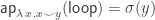
The name $\smile$ is suggestive – it satisfies most properties that you’d expect from a ‘cup product’ (in fact it induces a ‘true’ cup product via the map $\mathbb{S}^2 \to K(\mathbb{Z},2)$ ). It satisfies the following properties, all provable by circle induction:

$x \smile x = \mathsf{north}$
$x \smile y = - (y \smile x)$
$(- x) \smile y = -(x \smile y)$
$x \smile (x + y) = x \smile y$

This product induces an equivalence $\mathcal{F} : \mathbb{S}^1 * \mathbb{S}^1 \simeq \mathbb{S}^3$ by

$\mathcal{F} (\mathsf{inl}(x)) = \mathsf{north}$
$\mathcal{F} (\mathsf{inr}(x)) = \mathsf{north}$
$\mathsf{ap}_{\mathcal{F}} (\mathsf{push}(x,y)) = \sigma( x \smile y)$

That’s a really cute function! Its inverse isn’t, but let’s not bother with that now.

$\pi_3$ via joins

The reason the Brunerie map is so hard to analyse is because it is defined as the precomposition of a nice map $\beta_1 : \mathbb{S}^1 * \mathbb{S}^1 \to \mathbb{S}^2$ with a not so nice map, namely $\mathcal{F}^{-1} : \mathbb{S}^3 \to \mathbb{S}^1 * \mathbb{S}^1$ . However, what if we defined $\pi_3(\mathbb{S}^2) := |\!| \mathbb{S}^1 * \mathbb{S}^1 \to_* \mathbb{S}^2 |\!|_0$ instead? Clearly, this definition is equivalent to the usual one by precomposition with $\mathcal{F}$ . This would allow us redefine the Brunerie map to be simply $\beta_1$ and ignore that annoying precomposition with $\mathcal{F}^{-1}$ . Let’s make this happen.

For a pointed type $A$ , let us define

$\pi_3^*(A) := |\!| \mathbb{S}^1 * \mathbb{S}^1 \to_* A|\!|_0$

We can give this group an explicit multiplication. Given a function $f$ , we get an induced map $f^\Omega : \mathbb{S}^1 \times \mathbb{S}^1 \to \Omega \,A$ defined by

$f^\Omega(x,y) = \mathsf{ap}_f(\mathsf{push}(\mathsf{base},\mathsf{base}) \cdot \mathsf{push}(x,\mathsf{base})^{-1} \cdot \mathsf{push}(x,y) \cdot \mathsf{push}(\mathsf{base},y)^{-1})$

Looks horrible! Fortunately, the above tends to be equal to $\mathsf{ap}_f(\mathsf{push}(x,y))$ when $f$ is reasonable. The multiplication of two maps $f$ and $g$ in $\pi_3^*(A)$ is induced by the composition $f^\Omega(x,y) \cdot g^\Omega(x,y)$ .

It is relatively straightforward (at least if one assumes that $A$ is $1$ -connected) to show that $\mathcal{F}$ induces a group isomorphism $\pi_3(A) \cong \pi^*_3(A)$ . This is the key to understanding $\beta$ .

The proof

Now we’re ready to tackle the problem at hand. Recall that we have an equivalence $e : \pi_3(\mathbb{S}^2) \cong \mathbb{Z}$ . In the first 3 chapters of Brunerie’s thesis, he shows that $\pi_4(\mathbb{S}^3) \cong \mathbb{Z}/n \mathbb{Z}$ where $n = e(|\,\beta\,|)$ and where $\beta$ is the Brunerie map $\mathbb{S}^3 \to \mathbb{S}^2$ . It’s probably time to define $\beta$ . We’ll first need to actually define the aforementioned map $\beta_1 : \mathbb{S}^1 * \mathbb{S}^1 \to \mathbb{S}^2$ . We define it by:

$\beta_1(\mathsf{inl}(x)) = \mathsf{north}$
$\beta_1(\mathsf{inr}(y)) = \mathsf{north}$
$\mathsf{ap}_{\beta_1}(\mathsf{push}(x,y)) = \sigma(y) \cdot \sigma(x)$

The map $\beta$ is then just defined by $\beta = \beta_1 \circ \mathcal{F}^{-1}$ .

Note that the choice of equivalence $\pi_3(\mathbb{S}^2) \cong \mathbb{Z}$ does not matter — any two differ at most by a sign. Our job will therefore now be to construct a suitable equivalence $e : \pi_3(\mathbb{S}^2) \cong \mathbb{Z}$ and trace $\beta$ under it. We will see that when we land in $\mathbb{Z}$ , $\beta$ will have been mapped to $-2$ , establishing that the Brunerie number (well, our definition of it) is $-2$ . We achieve this by defining $e$ as a composition of 4 group isomorphisms $e_1,\dots,e_4$ and simultaneously tracing $\beta$ step by step.

$\underline{e_1 : \pi_3(\mathbb{S}^2) \cong \pi_3^*(\mathbb{S}^2)}$

This is defined by precomposition with $\mathcal{F}$ . By definition, $\beta$ gets mapped to $\beta_1$ .

$\underline{e_2 : \pi_3^(\mathbb{S}^2) \cong \pi_3^(\mathbb{S}^1 * \mathbb{S}^1)}$

I have not been able to come up with a concrete definition of the map $\pi_3^*(\mathbb{S}^2) \to \pi_3^*(\mathbb{S}^1 * \mathbb{S}^1)$ — it comes from the long exact sequence of homotopy groups induced from the Hopf fibration. Fortunately, however, its inverse is easy to describe: it is simply postcomposition with the Hopf map $h : \mathbb{S}^1 * \mathbb{S}^1 \to \mathbb{S}^2$ . The Hopf map is defined as follows:

$h(\mathsf{inl}(x)) = \mathsf{north}$
$h(\mathsf{inr}(y)) = \mathsf{north}$
$\mathsf{ap}_{h}(\mathsf{push}(x,y)) = \sigma(y - x)$

Let’s construct the element $\beta_2 : \mathbb{S}^1 * \mathbb{S}^1 \to \mathbb{S}^1 * \mathbb{S}^1$ such that $e_2(|\,\beta_1\,|) = | \beta_2 |$ . It is defined as follows:

$\beta_2(\mathsf{inl}(x)) = \mathsf{inr}(-x)$
$\beta_2(\mathsf{inr}(y)) = \mathsf{inr}(y)$
$\mathsf{ap}_{\beta_2}(\mathsf{push}(x,y)) = \mathsf{push}(y-x,-x)^{-1} \cdot \mathsf{push}(y-x,y)$

This looks pretty ad hoc, but the construction is chosen carefully. In order to show $e_2(|\,\beta_1\,|) = | \beta_2 |$ , we show $e_2^{-1}(|\,\beta_2\,|) = | \beta_1 |$ . For this, we need to show that $h \circ \beta_2 = \beta_1$ . I won’t do this here, but the proof is very direct. The idea is that the terms in the $\mathsf{push}$ -case are chosen precisely to take care of the $y-x$ appearing in the definition of the Hopf map.

$\underline{e_3 : \pi_3^(\mathbb{S}^1 \mathbb{S}^1) \cong \pi_3^*(\mathbb{S}^3)}$

This is where our construction of $\mathcal{F}$ kicks in. The isomorphism $e_3$ is defined by postcomposition with $\mathcal{F}$ . Let’s define $\beta_3 : \mathbb{S}^1 * \mathbb{S}^1 \to \mathbb{S}^3$ . It is defined by

$\beta_3(\mathsf{inl}(x)) = \mathsf{north}$
$\beta_3(\mathsf{inr}(x)) = \mathsf{north}$
$\mathsf{ap}_{\beta_3}(\mathsf{push}(x,y)) = \sigma(x \smile y)^{-1} \cdot \sigma (x \smile y)^{-1}$

I claim that $e_3(| \,\beta_2\, |) = | \, \beta_3\, |$ . To prove this, we need to show that $\mathcal{F} \circ \beta_2 = \beta_3$ . Let’s consider the definition of $\mathcal{F} \circ \beta_2$ (modulo some light rewriting):

$(\mathcal{F} \circ \beta_2)(\mathsf{inl}(x)) = \mathsf{north}$
$(\mathcal{F} \circ \beta_2)(\mathsf{inr}(x)) = \mathsf{north}$
$\mathsf{ap}_{\mathcal{F} \circ \beta_2}(\mathsf{push}(x)) = {\sigma((y - x) \smile (-x))}^{-1} \cdot \sigma((y - x) \smile y)$

So, $\mathcal{F} \circ \beta_2$ and $\beta_3$ agree definitionally on point constructors, and the push case is immediate by the properties of $\smile$ and the fact that $\sigma(- a) = \sigma(a)^{-1}$ .

$\underline{e_4 : \pi_3^*(\mathbb{S}^3) \cong \mathbb{Z}}$

Showing that $\beta_3$ maps to $-2$ under the obvious isomorphism $e_4 : \pi_3^*(\mathbb{S}^3) \cong \mathbb{Z}$ is straightforward. I won’t do this here, but the idea is that by following $-1$ under $e_4^{-1}$ , we see that $| \,\beta_3 \,| = e_4^{-1}(-1) \cdot e_4^{-1}(-1)$ . In fact, we can also show that (a slight rephrasing of) $\beta_3$ maps to $-2$ by normalisation in Cubical Agda!

Now we’re done! We have constructed an equivalence $e : \pi_3(\mathbb{S}^2) \cong \mathbb{Z}$ and shown that it maps $\beta$ to $-2$ . Hence, we get, by chapters 1–3 in Brunerie’s thesis, that $\pi_4(\mathbb{S}^3)$ is $\mathbb{Z}/2\mathbb{Z}$ .

A corollary

We know, by Chapters 1–3 in Brunerie’s thesis that the map $\beta$ is related to $\pi_4(\mathbb{S}^3)$ . But what if we had not read these chapters? The above argument is not by itself enough to show that $\pi_4(\mathbb{S}^3) \cong \mathbb{Z}/2\mathbb{Z}$ . However, it is enough to show that

If $\pi_4(\mathbb{S}^3) \not \cong 1$ , then $\pi_4(\mathbb{S}^3) \cong \mathbb{Z}/2\mathbb{Z}$

In other words, the fact that $\beta$ is mapped to $-2$ is enough to detect the $2$ -torsion in $\pi_4(\mathbb{S}^3)$ .

To see this, let us consider $\beta_1$ , the easier-to-work-with cousin of $\beta$ , again. There is a map very similar to $\beta_1$ with the two composites in the $\mathsf{push}$ -case flipped. Let’s call it $\theta$ . It is defined by

$\theta(\mathsf{inl}(x)) = \mathsf{north}$
$\theta(\mathsf{inr}(y)) = \mathsf{north}$
$\mathsf{ap}_{\theta}(\mathsf{push}(x,y)) = \sigma(x) \cdot \sigma(y)$

It is an easy lemma that $\theta$ is homotopic to the constant map $\mathbb{S}^1 * \mathbb{S}^1 \to_* \mathbb{S}^2$ . In other words, if we could flip the two path components in the definition of $\beta_1$ , we would have $\beta_1 = \theta = \mathsf{const}$ . Naturally, this is not possible. But what happens if we suspend the situation?

By the Fredenthal suspension theorem, postcomposition with $\sigma : \mathbb{S}^2 \to \Omega \mathbb{S}^3$ induces a surjection $\pi_3^*(\mathbb{S}^2) \to \pi_3^*(\Omega \mathbb{S}^3) \cong \pi_4(\mathbb{S}^3)$ . We can easily show that $\sigma \circ \theta = \sigma \circ \beta_1$ : for point constructors it holds definitionally and for the $\mathsf{push}$ -case, we are left to show

$\mathsf{ap}_{\sigma}(\sigma(x)) \cdot \mathsf{ap}_{\sigma}(\sigma(y)) = \mathsf{ap}_{\sigma}(\sigma(y)) \cdot \mathsf{ap}_{\sigma}(\sigma(x))$

But this time, we are allowed to flip the path components: we have landed in $\Omega^2 \mathbb{S}^3$ , and thus the Eckmann-Hilton argument applies, making the above equation hold. So the surjection $\pi_3^*(\mathbb{S}^2) \to \pi_4(\mathbb{S}^3)$ takes $\beta_1$ to the constant map, and hence $\pi_4(\mathbb{S}^3)$ must be a subgroup of $\mathbb{Z}/2\mathbb{Z}$ .

Formalisation

A formalisation of this proof in Cubical Agda is available here (for some reason, $\beta$ is called $\eta$ in the formalisation — sorry!). I suspect that the argument shouldn’t be much harder to formalise in standard Agda or Coq.

The second half of the file contains the proof by normalising $\beta_3$ . This, of course, relies on univalence and higher inductive types computing properly and should be doable in other cubical systems, but not in Book HoTT.

3 Responses to The Brunerie Number Is -2

Mike Shulman says:

13 June 2022 at 00:21

This is quite excellent! Congratulations! I’m still wrapping my head around it, but I have a couple of questions.

1. It feels funny to me to use a representable definition of homotopy groups in HoTT. It’s always seemed to me like the primitive notion of path-space supplied by identity types is easier to work with, indeed kind of the point. I wonder whether your representable definition of $\pi_3^*(A)$ using $S^1 * S^1$ can be transferred back to a “primitive” notion? (E.g., write out the universal property of maps out of $S^1 * S^1$ and re-express it entirely in terms of paths and higher paths in $A$ .) If so, how much of the calculation could be reformulated in such primitive language?

2. You say that it doesn’t matter which isomorphism $\pi_3(S^2)\cong \mathbb{Z}$ we use, since as long as it’s a group isomorphism there are only two choices and they differ by a sign. That’s certainly true if we only care about calculating $\pi_4(S^3)$ up to isomorphism, since $2$ and $-2$ generate the same subgroup of $\mathbb{Z}$ . But can’t one still ask whether your isomorphism is the same as the “canonical” one given by the usual definition of the Hopf fibration, and thus whether the “original” Brunerie number really is $2$ or $-2$ ? Presumably this depends on a choice made in the definition of the Hopf fibration, but it would still be interesting to know whether the “usual” choice leads to $2$ or $-2$ .

- Axel Ljungström says:
  
  13 June 2022 at 11:56
  
  Thanks for the comment:-)
  
  1. Yeah, this feels funny to me too. I always try to avoid the representable definition, but it does have its advantages (clearer correspondence to cohomology/cohomotopy groups of spheres for instance — not that I used that here, but in theory at least…)
  
  I think the most important thing with $\pi_3^*$ is not that it’s defined using joins, but the fact that it’s equivalent to $|\!| \mathbb{S}^1 \times \mathbb{S}^1 \to \Omega A | \! |_0$ (for this to really be an equivalent I think we need to also require pointedness in both arguments of the functions $\mathbb{S}^1 \times \mathbb{S}^1 \to \Omega A$ ) which I’m kind of using implicitly.
  
  However, I don’t think we want to simplify things more than this. The really neat thing about the $\pi_3*$ definition (actually, this should probably be $\pi_n^*$ for arbitrary $n$ but I haven’t formalised that yet) is precisely that it allows us to consider maps $\mathbb{S}^1 * \mathbb{S}^1 \to A$ as maps $\mathbb{S}^1 \times \mathbb{S}^1 \to \Omega \,A$ instead. As was the case in the proof, this often allows us to describe the map we’re considering in terms of $+ : \mathbb{S}^1 \times \mathbb{S}^1 \to \mathbb{S}^1$ and $\smile : \mathbb{S}^1 \times \mathbb{S}^1 \to \mathbb{S}^2$ . In particular, proving things about such maps boils down to proving things about $+$ and $\smile$ , which breaks everything into small and elementary lemmas. You can, of course, also translate everything and work entirely in something like $\Omega^3 \mathbb{S}^3$ , but then you have to deal with big terms involving annoying coherence paths.
  
  2. Yeah, this is true. A reasonable criterion for the isomorphism $\mathbb{Z} \cong \pi_3(\mathbb{S}^2)$ being the canonical one seems to me to be that $1$ gets mapped to the Hopf map $\mathbb{S}^3 \to \mathbb{S}^2$ . With my definition, this should be the case. However, the definition of the Hopf map depends on two things: the definition of the (‘pre’-) Hopf map $h : \mathbb{S}^1 * \mathbb{S}^1 \to \mathbb{S}^2$ and the definition of the equivalence $\mathcal{F} : \mathbb{S}^1 * \mathbb{S}^1 \simeq \mathbb{S}^3$ . For the Hopf map, I think my definition should agree with Guillaume’s. He describes it via the Hopf construction, so one has to work a bit to see that it actually unfolds to my definition — this is what I remember verifying in Agda at least, but I might have got a sign wrong somewhere. The equivalence $\mathcal{F} : \mathbb{S}^1 * \mathbb{S}^1 \simeq \mathbb{S}^3$ is also sensitive. I defined it in terms of $\smile$ whereas Guillaume defined it using a more general argument. I’m not sure that my definition agrees with his exactly, but think it does (both are defined, in some sense, by pattern matching on the left argument). If, however, I would’ve constructed $\smile$ via pattern matching on the right, the Hopf map would’ve been flipped. Assuming our definitions of $\mathcal{F}$ are different, that of course begs the question: which one is the canonical one? It actually seems to me that the Hopf map does not have a canonical definition in HoTT, in the sense of its classical counterpart.
  
Urs Schreiber says:

15 June 2022 at 12:35

Just to say that a prolific but anonymous and unresponsive contributor has recently created an nLab page on the topic, titled:

“homotopy groups of spheres in HoTT”
<ncatlab.org/nlab/show/homotopy+groups+of+spheres+in+HoTT

(maybe this was copied over from the now deprecated “homotopytheory” sub web?, I am not sure)

The page remains a little telegraphic, but it could serve a good service to anyone interested in the topic.

I have now added there a pointer to this blog entry here, but if anyone would like to add more material, please feel invited.

(Just be sure to leave a brief log message of what you did, and check out the nForum discussion regarding the page, [here](https://nforum.ncatlab.org/discussion/14559/homotopy-groups-of-spheres-in-hott/?Focus=99755#Comment_99755))

In particular, if or when there is any citable publication on the work reported here, it would be nice to add a reference on the nLab page.